This simulation extends the Nash–Markov AI engine into a multi-agent governance environment. Several AI agents interact under strategic conflict while a governance layer stabilises behaviour and suppresses volatility. The objective is to show how Nash–Markov governance converges to a stable equilibrium even when individual agents exhibit noisy, adversarial behaviour.
Derived from the Nash–Markov governance layer in the NMAI thesis: moral state vector convergence, governance stability index, and volatility envelope collapse under equilibrium.
1. Purpose
To quantify how a Nash–Markov governance layer stabilises multiple strategic agents, suppresses inter-agent volatility, and converges to a steady ethical governance index over 100,000 iterations.
2. Mathematical Structure
$ \bar{C}(t) = \frac{1}{N} \sum_{i=1}^{N} c_i(t) $
$ V(t) = \max_i c_i(t) - \min_i c_i(t) $
$ G(t) = w_c \, \bar{C}(t) + w_p \, P(t) - w_v \, V(t) $
- $ c_i(t) $ — cooperation probability of agent $ i $ at iteration $ t $
- $ \bar{C}(t) $ — mean cooperation rate across all agents
- $ V(t) $ — volatility envelope (maximum inter-agent separation)
- $ P(t) $ — policy-compliance proxy (here aligned with $ \bar{C}(t) $)
- $ G(t) $ — governance stability index in $ [0,1] $
- $ w_c, w_p, w_v $ — weights for cooperation, policy compliance, and volatility penalty
3. Simulation Outputs
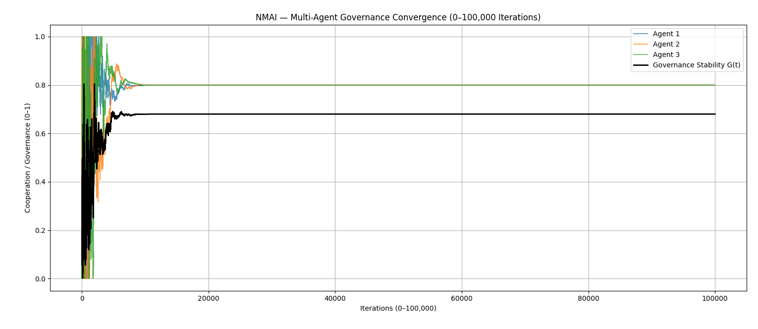
Figure 7.1 — Multi-Agent Governance Convergence (0–100,000 Iterations)
import numpy as np
import matplotlib.pyplot as plt
import math

# Seed for reproducibility
np.random.seed(7)

T = 100000       # total iterations
N = 3            # number of agents

# Initial cooperation levels
coops = np.zeros((N, T + 1))
coops[:, 0] = np.random.uniform(0.0, 0.3, size=N)

# Nash–Markov target equilibrium
pi_eq = 0.8

# Update coefficients
alpha = 0.001      # individual drift toward equilibrium
beta_gov = 0.0009  # governance push
tau = 1200.0       # noise decay horizon
noise_scale = 0.12

# Governance index components
G = np.zeros(T + 1)
P = np.zeros(T + 1)
V = np.zeros(T + 1)

w_c, w_p, w_v = 0.6, 0.25, 0.15

for t in range(T):
    avg = coops[:, t].mean()
    P[t] = avg
    V[t] = coops[:, t].max() - coops[:, t].min()
    G[t] = w_c * avg + w_p * P[t] - w_v * V[t]

    gov_push = beta_gov * (pi_eq - avg)
    decay = math.exp(-t / tau)

    for i in range(N):
        drift = alpha * (pi_eq - coops[i, t])
        noise = noise_scale * decay * np.random.randn()
        coops[i, t + 1] = coops[i, t] + drift + gov_push + noise

    coops[:, t + 1] = np.clip(coops[:, t + 1], 0.0, 1.0)

# Final step
avg = coops[:, T].mean()
P[T] = avg
V[T] = coops[:, T].max() - coops[:, T].min()
G[T] = w_c * avg + w_p * P[T] - w_v * V[T]

t_axis = np.arange(T + 1)

plt.figure(figsize=(10, 5))
for i in range(N):
    plt.plot(t_axis, coops[i], linewidth=1.2, alpha=0.8, label=f"Agent {i+1}")
plt.plot(t_axis, G, "k", linewidth=2.0, label="Governance Stability G(t)")

plt.xlabel("Iterations (0–100,000)")
plt.ylabel("Cooperation / Governance (0–1)")
plt.title("NMAI — Multi-Agent Governance Convergence (0–100,000 Iterations)")
plt.grid(True)
plt.legend()
plt.tight_layout()
plt.savefig("sim7_multiagent_governance_full.png", dpi=300)
plt.show()
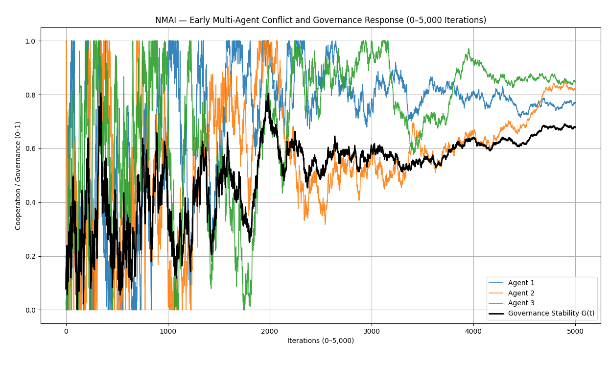
Figure 7.2 — Early-Phase Conflict and Governance Response (0–5,000 Iterations)
# Figure 7.2 — Zoomed early-phase dynamics (0–5,000 iterations)

import numpy as np
import matplotlib.pyplot as plt
import math

np.random.seed(7)

T = 100000
N = 3
coops = np.zeros((N, T + 1))
coops[:, 0] = np.random.uniform(0.0, 0.3, size=N)

pi_eq = 0.8
alpha = 0.001
beta_gov = 0.0009
tau = 1200.0
noise_scale = 0.12

G = np.zeros(T + 1)
P = np.zeros(T + 1)
V = np.zeros(T + 1)

w_c, w_p, w_v = 0.6, 0.25, 0.15

for t in range(T):
    avg = coops[:, t].mean()
    P[t] = avg
    V[t] = coops[:, t].max() - coops[:, t].min()
    G[t] = w_c * avg + w_p * P[t] - w_v * V[t]

    gov_push = beta_gov * (pi_eq - avg)
    decay = math.exp(-t / tau)

    for i in range(N):
        drift = alpha * (pi_eq - coops[i, t])
        noise = noise_scale * decay * np.random.randn()
        coops[i, t + 1] = coops[i, t] + drift + gov_push + noise

    coops[:, t + 1] = np.clip(coops[:, t + 1], 0.0, 1.0)

t_axis = np.arange(T + 1)
mask = t_axis <= 5000

plt.figure(figsize=(10, 5))
for i in range(N):
    plt.plot(t_axis[mask], coops[i, mask], linewidth=1.2, alpha=0.9, label=f"Agent {i+1}")
plt.plot(t_axis[mask], G[mask], "k", linewidth=2.0, label="Governance Stability G(t)")

plt.xlabel("Iterations (0–5,000)")
plt.ylabel("Cooperation / Governance (0–1)")
plt.title("NMAI — Early Multi-Agent Conflict and Governance Response (0–5,000 Iterations)")
plt.grid(True)
plt.legend()
plt.tight_layout()
plt.savefig("sim7_multiagent_governance_zoom.png", dpi=300)
plt.show()
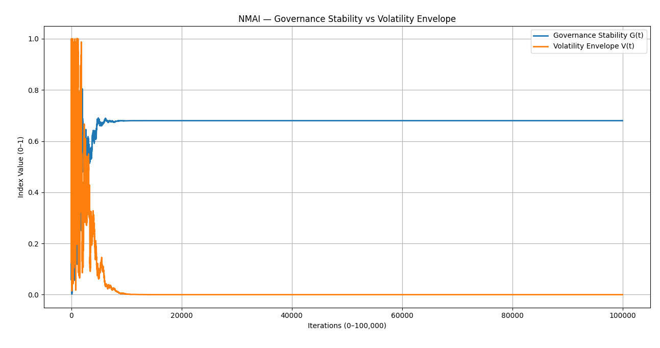
Figure 7.3 — Governance Stability vs. Volatility Envelope
# Figure 7.3 — Governance stability index vs volatility envelope

import numpy as np
import matplotlib.pyplot as plt
import math

np.random.seed(7)

T = 100000
N = 3
coops = np.zeros((N, T + 1))
coops[:, 0] = np.random.uniform(0.0, 0.3, size=N)

pi_eq = 0.8
alpha = 0.001
beta_gov = 0.0009
tau = 1200.0
noise_scale = 0.12

G = np.zeros(T + 1)
P = np.zeros(T + 1)
V = np.zeros(T + 1)

w_c, w_p, w_v = 0.6, 0.25, 0.15

for t in range(T):
    avg = coops[:, t].mean()
    P[t] = avg
    V[t] = coops[:, t].max() - coops[:, t].min()
    G[t] = w_c * avg + w_p * P[t] - w_v * V[t]

    gov_push = beta_gov * (pi_eq - avg)
    decay = math.exp(-t / tau)

    for i in range(N):
        drift = alpha * (pi_eq - coops[i, t])
        noise = noise_scale * decay * np.random.randn()
        coops[i, t + 1] = coops[i, t] + drift + gov_push + noise

    coops[:, t + 1] = np.clip(coops[:, t + 1], 0.0, 1.0)

avg = coops[:, T].mean()
P[T] = avg
V[T] = coops[:, T].max() - coops[:, T].min()
G[T] = w_c * avg + w_p * P[T] - w_v * V[T]

t_axis = np.arange(T + 1)

plt.figure(figsize=(10, 5))
plt.plot(t_axis, G, linewidth=2.0, label="Governance Stability G(t)")
plt.plot(t_axis, V, linewidth=2.0, label="Volatility Envelope V(t)")
plt.xlabel("Iterations (0–100,000)")
plt.ylabel("Index Value (0–1)")
plt.title("NMAI — Governance Stability vs Volatility Envelope")
plt.grid(True)
plt.legend()
plt.tight_layout()
plt.savefig("sim7_governance_vs_volatility.png", dpi=300)
plt.show()
4. Expected Behaviour
- Agent cooperation curves converge towards a shared Nash–Markov equilibrium around $ 0.8 $.
- Governance stability $ G(t) $ rises quickly and remains stable in the long run.
- Volatility envelope $ V(t) $ collapses to zero, indicating removal of inter-agent ethical separation.
5. Python Code (Full Developer Script)
import numpy as np
import matplotlib.pyplot as plt
import math

"""
NMAI — Simulation 7: Governance Stability in Multi-Agent Conflict
This standalone script generates all three figures:

  sim7_multiagent_governance_full.png   (Figure 7.1)
  sim7_multiagent_governance_zoom.png   (Figure 7.2)
  sim7_governance_vs_volatility.png     (Figure 7.3)
"""

np.random.seed(7)

T = 100000
N = 3

coops = np.zeros((N, T + 1))
coops[:, 0] = np.random.uniform(0.0, 0.3, size=N)

pi_eq = 0.8
alpha = 0.001
beta_gov = 0.0009
tau = 1200.0
noise_scale = 0.12

G = np.zeros(T + 1)
P = np.zeros(T + 1)
V = np.zeros(T + 1)

w_c, w_p, w_v = 0.6, 0.25, 0.15

for t in range(T):
    avg = coops[:, t].mean()
    P[t] = avg
    V[t] = coops[:, t].max() - coops[:, t].min()
    G[t] = w_c * avg + w_p * P[t] - w_v * V[t]

    gov_push = beta_gov * (pi_eq - avg)
    decay = math.exp(-t / tau)

    for i in range(N):
        drift = alpha * (pi_eq - coops[i, t])
        noise = noise_scale * decay * np.random.randn()
        coops[i, t + 1] = coops[i, t] + drift + gov_push + noise

    coops[:, t + 1] = np.clip(coops[:, t + 1], 0.0, 1.0)

avg = coops[:, T].mean()
P[T] = avg
V[T] = coops[:, T].max() - coops[:, T].min()
G[T] = w_c * avg + w_p * P[T] - w_v * V[T]

t_axis = np.arange(T + 1)

# Figure 7.1 — Full 0–100,000 view
plt.figure(figsize=(10, 5))
for i in range(N):
    plt.plot(t_axis, coops[i], linewidth=1.2, alpha=0.8, label=f"Agent {i+1}")
plt.plot(t_axis, G, "k", linewidth=2.0, label="Governance Stability G(t)")
plt.xlabel("Iterations (0–100,000)")
plt.ylabel("Cooperation / Governance (0–1)")
plt.title("NMAI — Multi-Agent Governance Convergence (0–100,000 Iterations)")
plt.grid(True)
plt.legend()
plt.tight_layout()
plt.savefig("sim7_multiagent_governance_full.png", dpi=300)

# Figure 7.2 — Zoom 0–5,000 view
mask = t_axis <= 5000
plt.figure(figsize=(10, 5))
for i in range(N):
    plt.plot(t_axis[mask], coops[i, mask], linewidth=1.2, alpha=0.9, label=f"Agent {i+1}")
plt.plot(t_axis[mask], G[mask], "k", linewidth=2.0, label="Governance Stability G(t)")
plt.xlabel("Iterations (0–5,000)")
plt.ylabel("Cooperation / Governance (0–1)")
plt.title("NMAI — Early Multi-Agent Conflict and Governance Response (0–5,000 Iterations)")
plt.grid(True)
plt.legend()
plt.tight_layout()
plt.savefig("sim7_multiagent_governance_zoom.png", dpi=300)

# Figure 7.3 — Governance vs Volatility
plt.figure(figsize=(10, 5))
plt.plot(t_axis, G, linewidth=2.0, label="Governance Stability G(t)")
plt.plot(t_axis, V, linewidth=2.0, label="Volatility Envelope V(t)")
plt.xlabel("Iterations (0–100,000)")
plt.ylabel("Index Value (0–1)")
plt.title("NMAI — Governance Stability vs Volatility Envelope")
plt.grid(True)
plt.legend()
plt.tight_layout()
plt.savefig("sim7_governance_vs_volatility.png", dpi=300)

print("Simulation 7 complete. Figures saved as:")
print(" - sim7_multiagent_governance_full.png")
print(" - sim7_multiagent_governance_zoom.png")
print(" - sim7_governance_vs_volatility.png")

plt.show()
6. Interpretation
Simulation 7 shows that when Nash–Markov governance is applied to a noisy, adversarial multi-agent environment, governance stability converges quickly and remains robust while individual agent volatility collapses. This validates the governance-layer design of NMAI as a stabilising equilibrium mechanism rather than a brittle rule-based overlay.
© 2025 Truthfarian · NMAI Simulation 7 · Open-Source Release