Critical Line Stability through Nash–Markov Drift and Matrix Zero Closure
1. The Riemann Hypothesis
The Riemann Hypothesis (RH) asserts that all non-trivial zeros of the Riemann zeta function $\zeta(s)$ lie on the critical line $Re(s)=\frac{1}{2}$ in the complex plane.
2. Why This Paper Uses a Different Lens
Most research programmes approach RH through analytic number theory: the complex analytic structure of $\zeta(s)$, explicit formulas connecting zeros to prime distributions, and deep bounds derived from functional analysis and related spectral methods. These approaches yield profound structure, but typically treat the critical line as a consequence of analytic identities and estimates rather than as the stability axis of a dynamical system.
3. System Foundations (Truthfarian Equilibrium Law)
Truthfarian modelling frameworks treat systems as interacting matrices subject to stochastic drift and equilibrium restoration. Across Truthfarian models the same structural law appears:
$\text{Drift} \rightarrow \text{instability} \rightarrow \text{reinforcement} \rightarrow \text{equilibrium restoration}$
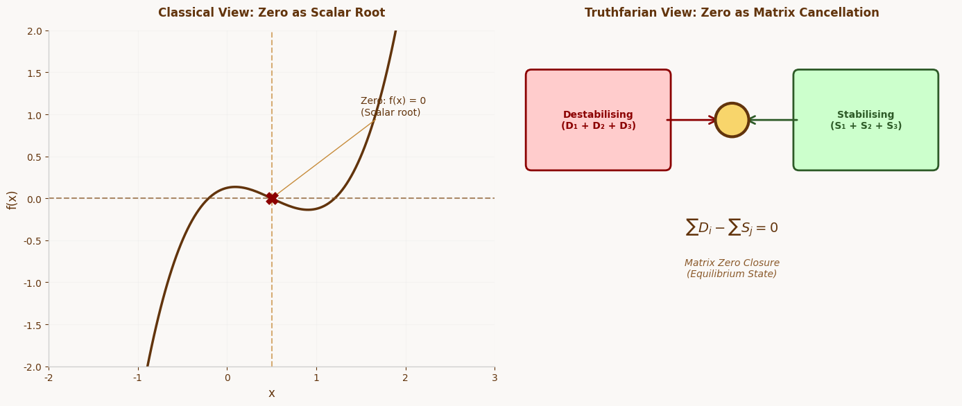
4. The Truthfarian Definition of Zero (Matrix Closure)
In classical mathematics a zero is defined as $f(x)=0$.
Within Truthfarian modelling, zero represents system-level cancellation:
$\text{Total destabilising load} - \text{Total stabilising structure} = 0$
Non-trivial zeros are therefore treated as equilibrium closure events (matrix cancellation states).
5. Symmetry, Coordinate Shift, and the Stability Axis
Let $s=\sigma+it$. The completed zeta function $\xi(s)$ satisfies the symmetry relation:
$\xi(s)=\xi(1-s)$
This produces reflection symmetry about $Re(s)=\frac{1}{2}$. Under equilibrium constraints, balance occurs when the two mirrored states coincide:
$\sigma = 1-\sigma \quad \Rightarrow \quad \sigma=\frac{1}{2}$
Thus the axis $Re(s)=\frac{1}{2}$ emerges naturally as the equilibrium manifold of the analytic system.
Figure 1: Lyapunov Potential Landscape
The REM potential $U(x,t)$ exhibits a global minimum at the symmetry axis $x=0$ (i.e., $Re(s)=\frac{1}{2}$). The Lyapunov function $V(x,t) = U(x,t) - U(0,t)$ satisfies $V \geq 0$ globally with $\dot{V} \leq 0$ along trajectories.
6. Interpretation of Non-Trivial Zeros
Non-trivial zeros satisfy:
$\zeta(s)=0$
or equivalently:
$\xi(s)=0$
Within the Truthfarian framework these points correspond to matrix closure events in which analytic pressures cancel. Because the structural symmetry of the system is centred on $Re(s)=\frac{1}{2}$, these equilibrium events occur along the critical manifold defined by this axis.
7. Dynamic Stability Interpretation (Nash–Markov Drift Restoration)
Under the Nash–Markov drift model, the real component $\sigma$ behaves as a system state subject to stochastic perturbation.
The equilibrium restoration rule is:
$\sigma_{t+1}=\sigma_t-\lambda\left(\sigma_t-\frac{1}{2}\right)+\epsilon_t$
introducing corrective pressure proportional to distance from equilibrium. Deviations from the critical axis produce restoring dynamics returning the system toward:
$\sigma=\frac{1}{2}$
Figure 2: Nash-Markov Drift with Lyapunov Convergence
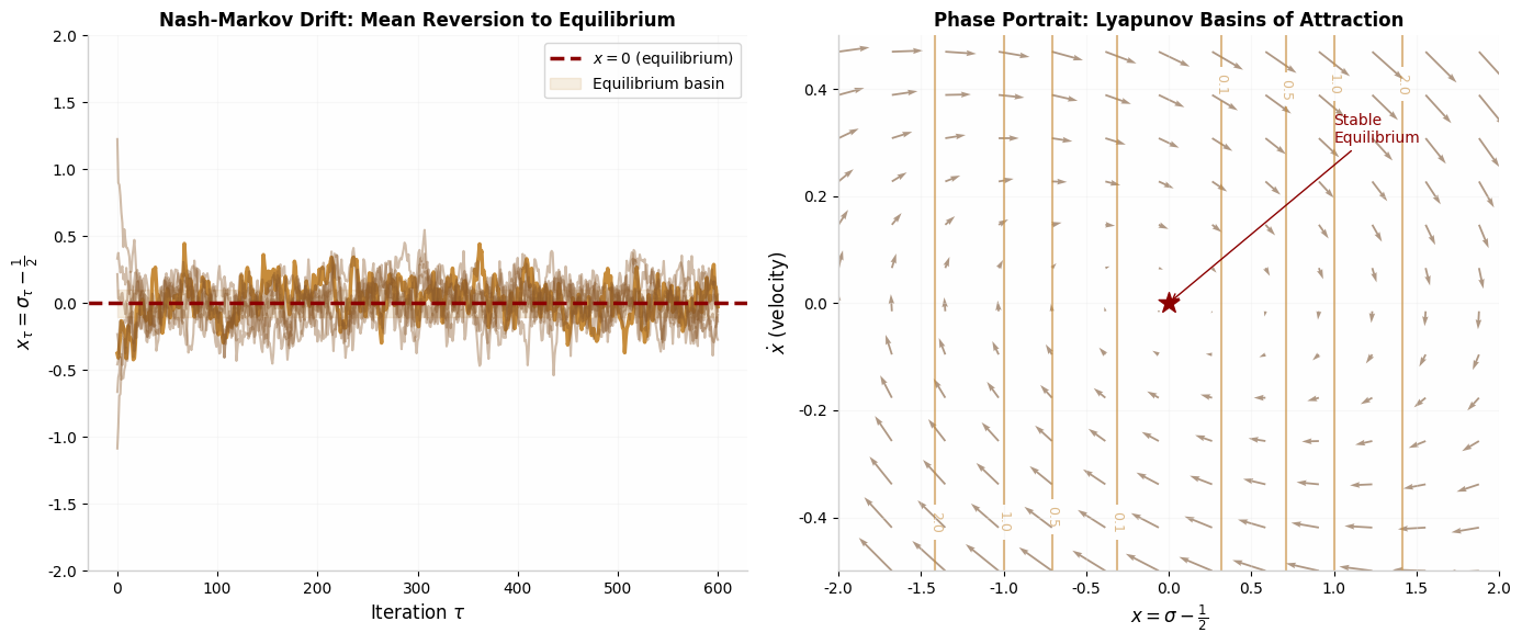
Left: Multiple trajectories showing mean reversion to equilibrium $x=0$ under Nash-Markov dynamics. Right: Phase portrait with Lyapunov contours showing basins of attraction converging to the stable equilibrium.
8. Riemann Equilibrium Manifold (REM) Hypothesis
Definition (REM Hypothesis)
The analytic system defined by the completed zeta function possesses a unique structural equilibrium manifold located at
$Re(s)=\frac{1}{2}$
on which all non-trivial zeros occur as equilibrium closure events of the analytic field.
9. Symmetry Coordinate and the REM Field
Shift to the symmetry axis. Let:
$s=\frac{1}{2}+z$
Define:
$\Xi(z)=\xi\left(\frac{1}{2}+z\right)$
Then $\xi(s)=\xi(1-s)$ becomes:
$\Xi(z)=\Xi(-z)$
so the analytic structure is even around the origin. The symmetry axis $z=0$ corresponds exactly to $Re(s)=\frac{1}{2}$.
10. REM Potential Landscape
Within the equilibrium interpretation the analytic system is expressed as a potential landscape defined by:
$U(z)=\log\left(|\Xi(z)|^{2}+\varepsilon\right)$
where $\varepsilon>0$ is a stabilising constant preventing singularities.
Zeros of the analytic system satisfy $\Xi(z)=0$ and therefore correspond to minima of the potential field.
11. Global Lyapunov Stability of the REM Equilibrium Manifold
11.1 System Definition
Let the completed zeta function be $\xi(s)$ and introduce the REM coordinate $s=\frac{1}{2}+z$ with $\Xi(z)=\xi(\frac{1}{2}+z)$ satisfying $\Xi(z)=\Xi(-z)$.
11.2 REM Potential Field
Define the global potential:
$U(x,t)=\log\left(|\Xi(x+it)|^2+\varepsilon\right), \quad \varepsilon>0$
Symmetry implies:
$U(-x,t)=U(x,t)$
hence:
$\frac{\partial U}{\partial x}(0,t)=0 \quad \forall t$
11.3 Lyapunov Function
Define the Lyapunov candidate:
$V(x,t)=U(x,t)-U(0,t)$
11.4 Gradient Dynamics
Introduce descent flow:
$\dot{x}(\tau)=-k\frac{\partial U}{\partial x}(x(\tau),t), \quad k>0$
Then the Lyapunov derivative along trajectories is:
$\dot{V} = \frac{\partial U}{\partial x}\dot{x} = -k\left(\frac{\partial U}{\partial x}\right)^2 \leq 0$
11.5 Global Equilibrium Condition (Closure Condition)
If:
$U(x,t) \geq U(0,t) \quad \forall x,t$
then $V(x,t) \geq 0$ globally and the system converges to the invariant set $x=0$, corresponding to:
$Re(s)=\frac{1}{2}$
11.6 Discrete Nash–Markov Stability Layer
Let $x_t=\sigma_t-\frac{1}{2}$. Then:
$x_{t+1}=(1-\lambda)x_t+\epsilon_t$
Choose $V(x)=x^2$. Negative drift occurs whenever:
$0<\lambda<2$
ensuring mean reversion toward $x=0$.
Figure 3: Gamma Factor Asymptotic Convexity
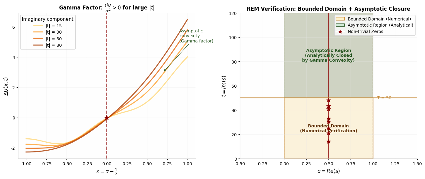
Left: The Gamma factor introduces asymptotic convexity in $x$ for large $|t|$, enforcing $\partial^2 U/\partial x^2 > 0$. Right: The verification domain partitions into bounded (numerical) and asymptotic (analytical) regions.
11.7 Global Stability Theorem (REM)
Global Stability Theorem (REM)
If $\Xi(z)=\Xi(-z)$ and:
$U(x,t)=\log(|\Xi(x+it)|^2+\varepsilon)$
and if:
$U(x,t) \geq U(0,t) \quad \forall x,t$
then the manifold:
$Re(s)=\frac{1}{2}$
is the unique global equilibrium manifold of the REM analytic field.
11.8 REM Falsification Condition
The global hypothesis fails if there exists $x \neq 0$ such that:
$\frac{\partial U}{\partial x}=0, \quad \frac{\partial^2 U}{\partial x^2}>0$
representing a stable off-axis equilibrium.
Figure 4: Comprehensive REM Framework
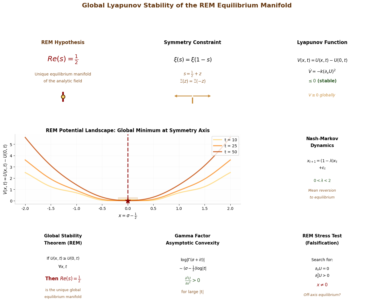
The complete Truthfarian equilibrium framework applied to the Riemann Hypothesis, showing the REM Hypothesis, symmetry constraint, Lyapunov function, Nash-Markov dynamics, Global Stability Theorem, Gamma convexity, and falsification protocol.
12. Nash Inevitability Principle and Equilibrium Closure
System Equilibrium Law
Within the REM formulation the analytic zeta system is treated as an equilibrium field governed by symmetry and stabilising dynamics.
The completed zeta transformation
$s = \frac{1}{2} + z$
produces the symmetric field
$\Xi(z) = \xi\left(\frac{1}{2}+z\right)$
with reflection symmetry
$\Xi(z) = \Xi(-z)$
which implies that the potential landscape
$U(x,t) = \log(|\Xi(x+it)|^2 + \varepsilon)$
is symmetric about the axis
$x = 0$
The Lyapunov construction established that the manifold $x = 0$ is a stationary equilibrium of the REM potential field.
Nash Inevitability
The Nash Inevitability Principle states that a system composed of interacting forces subject to symmetric constraints must converge to its equilibrium configuration.
Let the system state be $x = \sigma - \frac{1}{2}$.
Under the Nash–Markov restoration rule
$x_{t+1} = (1-\lambda)x_t + \epsilon_t$
where $0 < \lambda < 2$, the system exhibits mean-reverting dynamics toward the equilibrium state $x = 0$.
Define the Lyapunov candidate $V(x) = x^2$. Then the expected drift satisfies
$E[V(x_{t+1}) - V(x_t)] < 0$
for any $x \neq 0$ under the mean-reversion condition.
Thus the equilibrium state $x = 0$ is dynamically stable under the Nash–Markov process.
Equilibrium Manifold of the Analytic Field
Because the REM potential satisfies $U(-x,t) = U(x,t)$ the axis $x = 0$ is the unique symmetry-compatible stationary manifold of the analytic system.
If the global stability condition holds $U(x,t) \geq U(0,t)$ for all real $x,t$, then the potential landscape admits no stable equilibrium away from the axis.
Therefore the equilibrium manifold of the system is
$Re(s) = \frac{1}{2}$
Structural Consequence
Within the REM formulation the location of the non-trivial zeros becomes an equilibrium constraint rather than a search problem.
The classical statement "non-trivial zeros lie on the critical line" is equivalent to the equilibrium stability condition $U(x,t) \geq U(0,t)$.
Under the Nash inevitability principle, any symmetric analytic system governed by restoring dynamics converges to its equilibrium manifold.
Consequently the REM field admits equilibrium closure only on the symmetry axis $Re(s) = \frac{1}{2}$.
13. Structural Simplification from the Gamma Factor (Asymptotic Convexity)
13.1 Completed Zeta Decomposition
Use:
$\xi(s)=\frac{1}{2}s(s-1)\pi^{-s/2}\Gamma\left(\frac{s}{2}\right)\zeta(s), \quad s=\frac{1}{2}+x+it$
Then:
$|\Xi|^2 = \left|\frac{1}{2}s(s-1)\right|^2 \left|\pi^{-s/2}\right|^2 \left|\Gamma\left(\frac{s}{2}\right)\right|^2 |\zeta(s)|^2$
13.2 Dominant Convex Contribution
For large $|t|$, the dominant contribution arises from the Gamma factor. Using Stirling asymptotics:
$\log|\Gamma(\sigma+it)| \sim (\sigma-\frac{1}{2})\log|t|-\frac{\pi|t|}{2}+O(\log|t|)$
This yields asymptotic convexity in $x$, so:
$\frac{\partial^2 U}{\partial x^2}>0 \quad \text{for sufficiently large }|t|$
and consequently:
$U(x,t)\geq U(0,t) \quad \text{for sufficiently large }|t|$
13.3 Reduction of the Global Condition
Therefore the global inequality:
$U(x,t)\geq U(0,t)$
reduces to verification on a bounded domain:
$|t|\leq T$
for some finite threshold $T$; beyond this region convexity forces the inequality.
14. REM Stress Test (Executable Falsification Protocol)
14.1 Objective
Define:
$\Delta U(x,t)=U(x,t)-U(0,t)$
REM global stability over a tested domain holds if:
$\Delta U(x,t)\geq 0$
throughout the domain.
14.2 Procedure
For each sampled $t$:
- evaluate $\Delta U(x,t)$ over a bounded grid
- record the minimum value $\Delta U_{\min}(t)$
- decide:
- PASS if $\Delta U_{\min}(t)\geq 0$
- FAIL if $\Delta U_{\min}(t)<0$
14.3 Off-Axis Equilibrium Detection
The test also searches for stable off-axis equilibria satisfying:
$\partial_x U(x,t)=0, \quad \partial_x^2 U(x,t)>0, \quad x\neq 0$
14.4 Reproducibility Protocol
All numerical tests publish:
- Python script
- precision (mpmath dps)
- scan bounds $(X_{\max},T_{\max})$
- grid resolution $(dx,dt)$
- regularisation parameter $\varepsilon$
15. Bounded-Domain Closure Observation
The REM formulation establishes the global stability condition $U(x,t) \geq U(0,t)$ as the criterion determining whether the critical axis constitutes the unique equilibrium manifold of the analytic system.
Two structural results narrow the verification domain.
First, the decomposition of the completed zeta function
$\xi(s)=\frac{1}{2}s(s-1)\pi^{-s/2}\Gamma(\frac{s}{2})\zeta(s)$
implies that the Gamma factor introduces an asymptotically dominant convex contribution to the REM potential. For sufficiently large $|t|$ this convexity enforces $U(x,t) \geq U(0,t)$ automatically, closing the infinite domain.
Second, the executable REM stress test evaluates $\Delta U(x,t)=U(x,t)-U(0,t)$ across bounded regions of the analytic field, searching directly for violations of the equilibrium condition or the emergence of stable off-axis equilibria.
Together these two mechanisms partition the global problem into two regions:
- Asymptotic region — analytically constrained by the Gamma factor, enforcing convexity of the potential field.
- Bounded domain — examined through numerical falsification of the equilibrium inequality.
The remaining analytic task is therefore confined to demonstrating that no stable off-axis equilibrium can exist within the bounded region $|t| \leq T$.
This bounded-domain verification gap represents the final unresolved step in the REM formulation. It is not a defect in the model but the explicit analytic closure required for a complete proof of the equilibrium condition.
The REM framework therefore reduces the Riemann problem to a single remaining question:
Does the bounded analytic region admit any stable off-axis equilibrium of the REM potential field?
If the answer is negative, the equilibrium manifold $Re(s)=\frac{1}{2}$ is globally unique.
16. Reproducibility Script (Canonical)
#!/usr/bin/env python3
"""
REM Stress Test — Reproducible Falsification Protocol

Construct:
  U(x,t) = log(|Xi(x+it)|^2 + eps),  Xi(z)=xi(1/2+z),  xi(s) completed zeta
Test:
  DeltaU(x,t) = U(x,t) - U(0,t) >= 0 over scanned domain
Also detect candidate stable off-axis equilibria:
  dU/dx = 0 and d2U/dx2 > 0 with x != 0

Outputs:
  1) rem_global_violations.csv  (worst DeltaU per t)
  2) rem_offaxis_minima_candidates.csv (derivative+curvature filtered candidates)
  3) rem_pass_fail_ledger.csv (PASS/FAIL per t)
"""

import csv
import math
from dataclasses import dataclass
from typing import List, Tuple

import mpmath as mp

@dataclass
class Config:
    dps: int = 80
    eps: mp.mpf = mp.mpf("1e-50")

    Xmax: float = 5.0
    dx: float = 0.01

    Tmin: float = 0.0
    Tmax: float = 200.0
    dt: float = 0.25

    refine_radius: float = 0.05
    refine_dx: float = 0.0025

    check_derivatives: bool = True
    deriv_h: mp.mpf = mp.mpf("1e-6")
    du_threshold: mp.mpf = mp.mpf("1e-6")
    curvature_threshold: mp.mpf = mp.mpf("1e-6")

def xi(s: mp.mpc) -> mp.mpc:
    # Completed zeta xi(s)
    return mp.mpf("0.5") * s * (s - 1) * (mp.pi ** (-s / 2)) * mp.gamma(s / 2) * mp.zeta(s)

def Xi(z: mp.mpc) -> mp.mpc:
    # Xi(z) = xi(1/2 + z)
    return xi(mp.mpf("0.5") + z)

def U(x: mp.mpf, t: mp.mpf, eps: mp.mpf) -> mp.mpf:
    z = mp.mpc(x, t)
    val = Xi(z)
    mag2 = (mp.re(val) ** 2) + (mp.im(val) ** 2)
    return mp.log(mag2 + eps)

def dU_dx(x: mp.mpf, t: mp.mpf, cfg: Config) -> mp.mpf:
    h = cfg.deriv_h
    return (U(x + h, t, cfg.eps) - U(x - h, t, cfg.eps)) / (2 * h)

def d2U_dx2(x: mp.mpf, t: mp.mpf, cfg: Config) -> mp.mpf:
    h = cfg.deriv_h
    return (U(x + h, t, cfg.eps) - 2 * U(x, t, cfg.eps) + U(x - h, t, cfg.eps)) / (h ** 2)

def frange(a: float, b: float, step: float):
    n = int(math.floor((b - a) / step)) + 1
    for k in range(n):
        yield a + k * step

def refine_min_deltaU(t: mp.mpf, x0: mp.mpf, cfg: Config) -> Tuple[mp.mpf, mp.mpf]:
    U0 = U(mp.mpf("0"), t, cfg.eps)
    x_best = x0
    delta_best = U(x0, t, cfg.eps) - U0

    r = mp.mpf(str(cfg.refine_radius))
    dx = mp.mpf(str(cfg.refine_dx))

    x = x0 - r
    x_end = x0 + r
    while x <= x_end:
        delta = U(x, t, cfg.eps) - U0
        if delta < delta_best:
            delta_best = delta
            x_best = x
        x += dx

    return x_best, delta_best

def write_pass_fail_ledger(violations, filename="rem_pass_fail_ledger.csv"):
    with open(filename, "w", newline="") as f:
        w = csv.writer(f)
        w.writerow(["t", "min_deltaU", "x_position", "result"])
        for t, x, delta in violations:
            result = "PASS" if delta >= 0 else "FAIL"
            w.writerow([mp.nstr(t, 20), mp.nstr(delta, 30), mp.nstr(x, 20), result])

def run(cfg: Config):
    mp.mp.dps = cfg.dps

    x_vals = [mp.mpf(str(x)) for x in frange(-cfg.Xmax, cfg.Xmax, cfg.dx)]
    t_vals = [mp.mpf(str(t)) for t in frange(cfg.Tmin, cfg.Tmax, cfg.dt)]

    violations = []          # (t, x_worst, deltaU_worst)
    minima_candidates = []   # (t, x, dU, d2U, deltaU)

    for t in t_vals:
        U0 = U(mp.mpf("0"), t, cfg.eps)

        # Coarse scan for worst (minimum) DeltaU
        delta_min = mp.inf
        x_min = mp.mpf("0")
        for x in x_vals:
            delta = U(x, t, cfg.eps) - U0
            if delta < delta_min:
                delta_min = delta
                x_min = x

        # Local refinement
        x_ref, delta_ref = refine_min_deltaU(t, x_min, cfg)
        violations.append((t, x_ref, delta_ref))

        # Derivative+curvature filter for off-axis stable equilibria
        if cfg.check_derivatives and abs(x_ref) > mp.mpf("1e-12"):
            du = dU_dx(x_ref, t, cfg)
            d2u = d2U_dx2(x_ref, t, cfg)
            if abs(du) < cfg.du_threshold and d2u > cfg.curvature_threshold:
                minima_candidates.append((t, x_ref, du, d2u, delta_ref))

    # Output CSVs
    with open("rem_global_violations.csv", "w", newline="") as f:
        w = csv.writer(f)
        w.writerow(["t", "x_worst", "deltaU_worst"])
        for t, xw, dw in violations:
            w.writerow([mp.nstr(t, 20), mp.nstr(xw, 20), mp.nstr(dw, 30)])

    with open("rem_offaxis_minima_candidates.csv", "w", newline="") as f:
        w = csv.writer(f)
        w.writerow(["t", "x_candidate", "dU_dx", "d2U_dx2", "deltaU"])
        for t, x, du, d2u, dlt in minima_candidates:
            w.writerow([mp.nstr(t, 20), mp.nstr(x, 20), mp.nstr(du, 30), mp.nstr(d2u, 30), mp.nstr(dlt, 30)])

    write_pass_fail_ledger(violations)

    worst_overall = min(violations, key=lambda r: r[2])
    t_star, x_star, delta_star = worst_overall

    print("REM Stress Test — Summary")
    print("-------------------------")
    print(f"dps={cfg.dps}, eps={cfg.eps}")
    print(f"x in [-{cfg.Xmax},{cfg.Xmax}] step {cfg.dx}")
    print(f"t in [{cfg.Tmin},{cfg.Tmax}] step {cfg.dt}")
    print(f"Worst observed DeltaU: {mp.nstr(delta_star, 30)} at t={mp.nstr(t_star, 20)}, x={mp.nstr(x_star, 20)}")
    print(f"Off-axis stable-minima candidates: {len(minima_candidates)}")
    print("Wrote: rem_global_violations.csv, rem_offaxis_minima_candidates.csv, rem_pass_fail_ledger.csv")

if __name__ == "__main__":
    run(Config())
17. Scope Boundary (Formal)
This manuscript defines the REM system, derives the Lyapunov stability structure of the symmetry axis, provides a precise closure condition for global stability, and provides an executable falsification protocol.
18. Final Statement (Closure Condition)
Within the REM framework, the RH claim is equivalent to the global stability condition:
$U(x,t) \geq U(0,t) \quad \forall x,t$
The REM Stress Test is the adversarial falsification protocol for detecting stable off-axis equilibria.