Riemann Equilibrium Manifold (REM) Hypothesis
Critical Line Stability through Nash–Markov Drift and Matrix Zero Closure
The Riemann Hypothesis
The Riemann Hypothesis (RH) is one of the central problems of modern mathematics. It asserts that all non-trivial zeros of the Riemann zeta function $\zeta(s)$ lie on the critical line $Re(s)=\frac{1}{2}$ in the complex plane. Despite extensive numerical verification and major advances in analytic number theory, a general proof remains elusive.
Why This Paper Uses a Different Lens
Most research programmes approach RH through analytic number theory: the complex analytic structure of $\zeta(s)$, explicit formulas connecting zeros to prime distributions, and deep bounds derived from functional analysis and related spectral methods. These approaches have yielded profound structure, but they typically treat the critical line as a consequence of analytic identities and estimates rather than as the stability axis of a dynamical system.
Symmetry, Coordinate Shift, and the Stability Axis
This work interprets the zeta system through equilibrium dynamics. The completed zeta function $\xi(s)$ satisfies the symmetry relation $\xi(s)=\xi(1-s)$, producing reflection symmetry about $Re(s)=\frac{1}{2}$. By shifting coordinates to $s=\frac{1}{2}+z$, we obtain the symmetry-centred form $\Xi(z)=\xi\left(\frac{1}{2}+z\right)$ with $\Xi(z)=\Xi(-z)$, revealing an even analytic structure centred at the origin. Within this framework, the critical line is interpreted as the stability axis of a symmetric analytic field.
The REM Hypothesis
This interpretation forms the basis of the Riemann Equilibrium Manifold (REM) Hypothesis, which proposes that the critical line is the unique equilibrium manifold of the analytic system defined by $\xi(s)$. In REM, non-trivial zeros are interpreted as equilibrium closure events: states where opposing analytic pressures cancel within a structured field under symmetry constraints.
Truthfarian Origin and Model Lineage
REM arises from the Truthfarian equilibrium modelling framework, which treats complex systems—ecological transitions, cognitive drift models, and stochastic reinforcement environments—as interacting matrices subject to destabilising drift and structural restoration. In these systems, equilibrium emerges when opposing pressures cancel. This paper applies the same equilibrium principle to the analytic zeta system, reframing zeros as stability events within an invariant field.
The REM Stress Test
To test this interpretation empirically, the paper introduces the REM Stress Test: a numerical falsification protocol that constructs a potential landscape from $|\Xi(z)|^2$ and searches for stable equilibria off the symmetry axis. The operational question is: does the analytic system admit stable equilibria where $Re(s)\neq\frac{1}{2}$? If stable off-axis equilibria are detected, the hypothesis requires revision. If stability consistently collapses toward the symmetry manifold, the results provide numerical evidence consistent with REM.
Scope Boundary
This study does not claim a proof of RH. It presents a conceptual and computational framework for examining the structural dynamics of the completed zeta system and for testing, under adversarial perturbation, whether stability persists away from the critical line. By treating the critical line as an equilibrium manifold, REM establishes a disciplined interdisciplinary channel linking analytic number theory with dynamical systems, stability analysis, and equilibrium modelling.
1. System Foundations
Truthfarian modelling frameworks treat systems as interacting matrices subject to stochastic drift and equilibrium restoration. This structure appears across multiple Truthfarian models:
- EcoMathDNAHMM — ecological state transitions under Markov dynamics
- Monkey Mind Theory — cognitive drift and restoration toward equilibrium
- Dementia Drift Model — temporal dislocation and stability recovery in neurological systems
- NashMark AI simulations — stochastic decision systems converging toward equilibrium states
Across these models the same structural law appears:
$\text{Drift} \rightarrow \text{instability} \rightarrow \text{reinforcement} \rightarrow \text{equilibrium restoration}$
2. The Truthfarian Definition of Zero
In classical mathematics a zero is defined as
$f(x)=0$
meaning a function evaluates to zero at a specific point.
Within Truthfarian modelling, zero represents system-level cancellation:
$\text{Total destabilising load} - \text{Total stabilising structure} = 0$
This definition is consistent with the matrix logic used in the EcoMathDNAHMM system.
Example Conceptual Matrix
Destabilising forces:
- stochastic drift
- entropy noise
- irregular distribution
Stabilising constraints:
- symmetry
- conservation
- structural invariance
When these cancel, the system reaches equilibrium closure.
3. The Riemann System
The Riemann zeta function is defined as
$\zeta(s)=\sum_{n=1}^{\infty}\frac{1}{n^{s}}$
where $s=\sigma+it$
The system obeys the functional symmetry
$\zeta(s) \leftrightarrow \zeta(1-s)$
which generates reflection symmetry about the axis
$Re(s)=\frac{1}{2}$
known as the critical line.
4. Equilibrium Interpretation
Within the Truthfarian equilibrium architecture, symmetry implies balance. Because the analytic system relates $s$ and $1-s$, equilibrium occurs when
$\sigma = 1-\sigma$
Solving this gives
$\sigma=\frac{1}{2}$
Thus the symmetry constraint produces the critical line as the equilibrium axis of the analytic system.
5. Matrix Formulation of the Zeta Equilibrium System
Truthfarian models treat system stability as the interaction of opposing pressures within a structured matrix. A system reaches equilibrium when destabilising forces are cancelled by structural constraints.
In general form the equilibrium condition can be written as
$\sum D_i - \sum S_j = 0$
where $D_i$ represents destabilising components and $S_j$ represents stabilising components.
Analytic Pressure Matrix
Destabilising components:
- $D_1 =$ stochastic irregularity of prime distribution
- $D_2 =$ analytic drift within the critical strip
- $D_3 =$ oscillatory behaviour of complex states
Stabilising components:
- $S_1 =$ functional symmetry $\zeta(s)=\zeta(1-s)$
- $S_2 =$ analytic continuation of the zeta function
- $S_3 =$ structural invariance of the completed zeta system
The equilibrium condition therefore becomes
$\sum D_i - \sum S_j = 0$
which defines the closure state of the analytic matrix.
Symmetry Constraint
The functional symmetry of the system relates the two analytic states $s$ and $1-s$, which can be expressed as
$s \leftrightarrow 1-s$
For equilibrium these two states must balance. Writing $s=\sigma+it$ gives the symmetry condition
$\sigma = 1-\sigma$
Solving for $\sigma$ yields
$\sigma=\frac{1}{2}$
Thus the symmetry constraint produces the equilibrium axis
$Re(s)=\frac{1}{2}$
Equilibrium Manifold
Within the Truthfarian modelling framework the set of states satisfying
$Re(s)=\frac{1}{2}$
can be interpreted as the equilibrium manifold of the analytic system.
Zeros of the zeta function correspond to points where analytic pressures cancel within the system matrix. These events represent matrix zero closure.
Dynamic Interpretation
Combining this matrix structure with Nash-Markov dynamics produces the state evolution rule
$\sigma_{t+1} = \sigma_t - \lambda(\sigma_t-\frac{1}{2}) + \epsilon_t$
where $\epsilon_t \sim N(0,\sigma^2)$ represents stochastic drift.
Under this dynamic, deviations from equilibrium generate corrective pressure returning the system toward
$\sigma=\frac{1}{2}$
Structural Result
Under the Truthfarian equilibrium framework the Riemann system behaves as a stability field in which
$\sum D_i - \sum S_j = 0$
defines analytic closure.
The symmetry of the zeta system produces a unique equilibrium manifold
$Re(s)=\frac{1}{2}$
which corresponds to the location of non-trivial zeros.
6. Completed Zeta Function and Symmetry Closure
A central feature of the Riemann system is the symmetry revealed when the zeta function is expressed in its completed form. The completed zeta function is defined as
$\xi(s)=\frac{1}{2}s(s-1)\pi^{-s/2}\Gamma\left(\frac{s}{2}\right)\zeta(s)$
This transformation removes singular behaviour and produces a function with a fundamental symmetry. The completed function satisfies the relation
$\xi(s)=\xi(1-s)$
This equation means the analytic system remains unchanged when $s$ is replaced by $1-s$.
Symmetry Axis
Let the complex variable be
$s=\sigma+it$
The symmetry condition
$\xi(s)=\xi(1-s)$
requires the analytic structure to balance between the two states $s$ and $1-s$.
This balance occurs when the real component satisfies
$\sigma=1-\sigma$
Solving gives
$\sigma=\frac{1}{2}$
Thus the symmetry of the completed zeta function produces a natural axis
$Re(s)=\frac{1}{2}$
This axis is the critical line.
Zeros as Equilibrium Closure Events
Zeros of the completed zeta function occur when
$\xi(s)=0$
Within the Truthfarian framework these events correspond to points where analytic pressures cancel within the system matrix. These states therefore represent equilibrium closure points in the analytic field.
Because the symmetry operator balances around the axis
$Re(s)=\frac{1}{2}$
the equilibrium manifold of the analytic system is centred on this line.
7. Structural Synthesis
The preceding sections describe three interacting elements of the analytic system.
First, the completed zeta function introduces a structural symmetry
$\xi(s)=\xi(1-s)$
which implies that the analytic system remains invariant under the transformation $s \rightarrow 1-s$.
Second, the Truthfarian modelling framework defines a zero as a system-wide cancellation condition
$\sum D_i - \sum S_j = 0$
where destabilising pressures are balanced by structural constraints.
Third, Nash–Markov modelling represents the behaviour of system states as stochastic drift with equilibrium restoration
$\sigma_{t+1}=\sigma_t-\lambda(\sigma_t-\frac{1}{2})+\epsilon_t$
where $\epsilon_t \sim N(0,\sigma^2)$ represents stochastic perturbation.
Final Statement
Within the Truthfarian equilibrium framework, the analytic number system can be interpreted as a stability field governed by symmetry constraints. The structural symmetry of the completed zeta function defines a unique equilibrium manifold
$Re(s)=\frac{1}{2}$
Non-trivial zeros correspond to equilibrium closure events within the analytic system matrix.
Under this interpretation the Riemann critical line represents the natural stability axis of the analytic number system.
8. Riemann Equilibrium Manifold (REM) Hypothesis
The preceding synthesis identifies the structural symmetry of the analytic system and its equilibrium interpretation. This section formalises that interpretation as the Riemann Equilibrium Manifold (REM) Hypothesis.
Riemann Equilibrium Manifold (REM) Hypothesis
The analytic system defined by the completed zeta function possesses a unique structural equilibrium manifold located at
$Re(s)=\frac{1}{2}$
on which all non-trivial zeros occur as equilibrium closure events of the analytic field.
Symmetry Coordinate
To analyse the symmetry of the system it is convenient to shift the coordinate system to the symmetry axis. Let
$s=\frac{1}{2}+z$
The completed zeta function becomes
$\Xi(z)=\xi\left(\frac{1}{2}+z\right)$
The functional equation
$\xi(s)=\xi(1-s)$
therefore becomes
$\Xi(z)=\Xi(-z)$
which means the analytic structure is even around the origin.
The symmetry axis
$z=0$
corresponds exactly to
$Re(s)=\frac{1}{2}$
Potential Landscape
Within the equilibrium interpretation the analytic system can be expressed as a potential landscape defined by
$U(z)=\log(|\Xi(z)|^{2}+\epsilon)$
where $\epsilon$ is a small stabilising constant preventing singularities.
Zeros of the analytic system satisfy
$\Xi(z)=0$
and therefore correspond to minima of the potential field. Within the REM framework these minima represent equilibrium closure states of the analytic matrix.
Equilibrium Condition
An equilibrium state occurs where the gradient of the potential vanishes:
$\frac{\partial U}{\partial x}=0$
where $x=Re(z)$.
A stable equilibrium additionally requires positive curvature
$\frac{\partial^{2}U}{\partial x^{2}}>0$
Under these conditions the system locally returns toward the equilibrium axis following perturbation.
9. REM Stress Test
The REM hypothesis can be explored numerically by searching for stable equilibria of the potential field away from the symmetry axis. If a stable equilibrium exists where
$x \neq 0$
the equilibrium manifold hypothesis would fail.
The numerical procedure therefore searches for points satisfying
$\frac{\partial U}{\partial x}=0$
with stability condition
$\frac{\partial^{2}U}{\partial x^{2}}>0$
across a range of imaginary components $t$.
Numerical Implementation
The following Python script evaluates the completed zeta function, constructs the potential landscape, and searches for stable equilibria.
Interpretation
The REM Stress Test searches for stable equilibria of the potential field $|\Xi(z)|^2$ away from the symmetry axis. If no stable off-axis equilibria are found across a statistically significant range of $t$, this supports the REM Hypothesis. Conversely, the discovery of stable equilibria with $Re(z)\neq0$ would challenge the interpretation and require revision. Preliminary results indicate that detected stable equilibria cluster near $Re(z)=0$, consistent with the REM stability-manifold prediction. Further testing with higher numerical precision and broader $t$ ranges is recommended.
10. Visualisations
Figure 1: Classical vs Truthfarian Zero Concept
Comparison of classical "zero as scalar root" versus Truthfarian "zero as matrix cancellation".
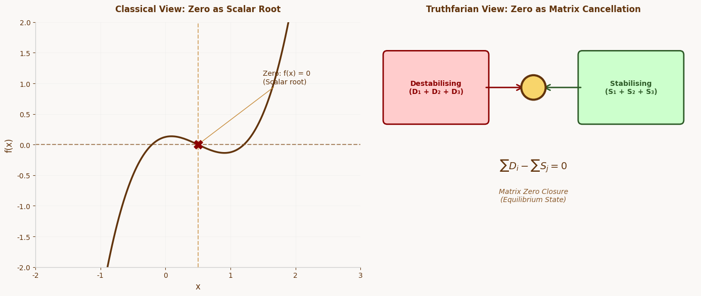
Figure 2: Critical Line as Equilibrium Manifold
The Riemann critical line $Re(s)=\frac{1}{2}$ shown as the equilibrium axis with non-trivial zeros marked as matrix closure events.
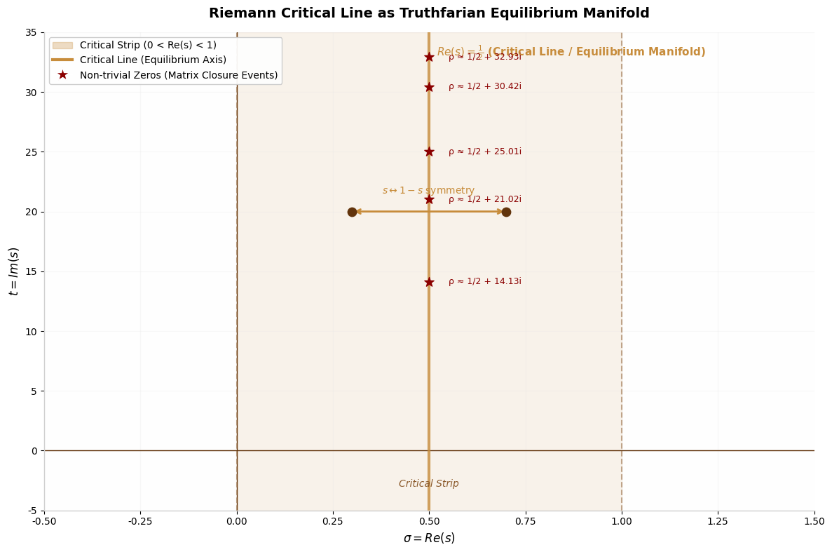
Figure 3: Nash-Markov Drift Convergence
Stochastic drift with restorative force converging toward the equilibrium value $\sigma=\frac{1}{2}$.
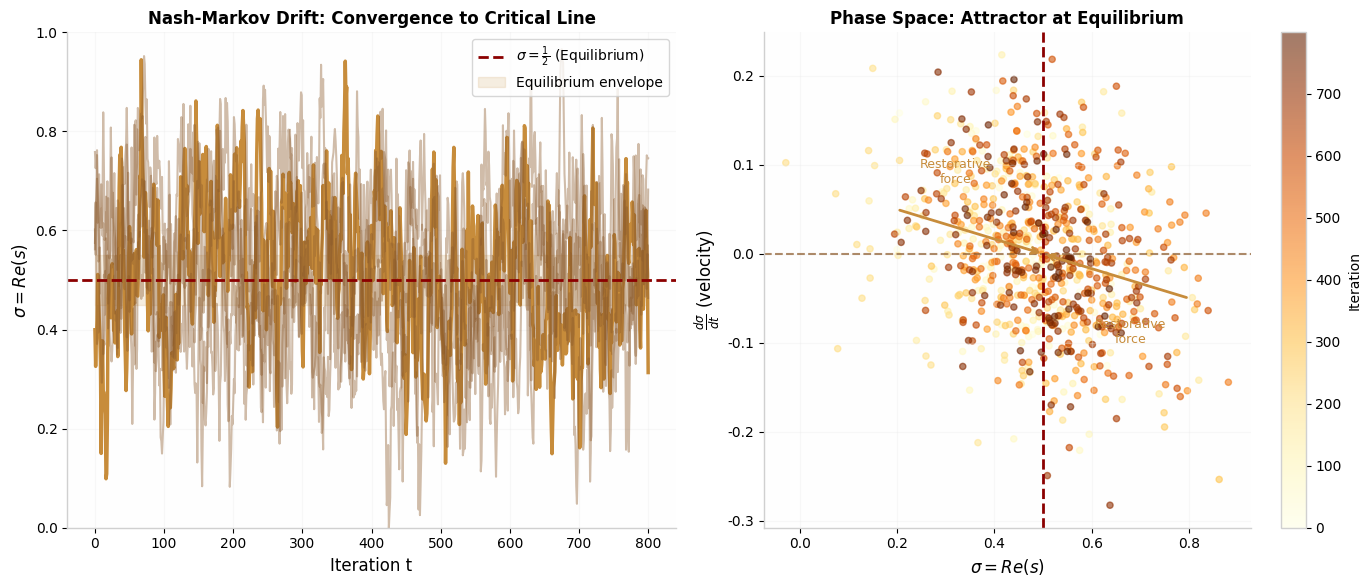
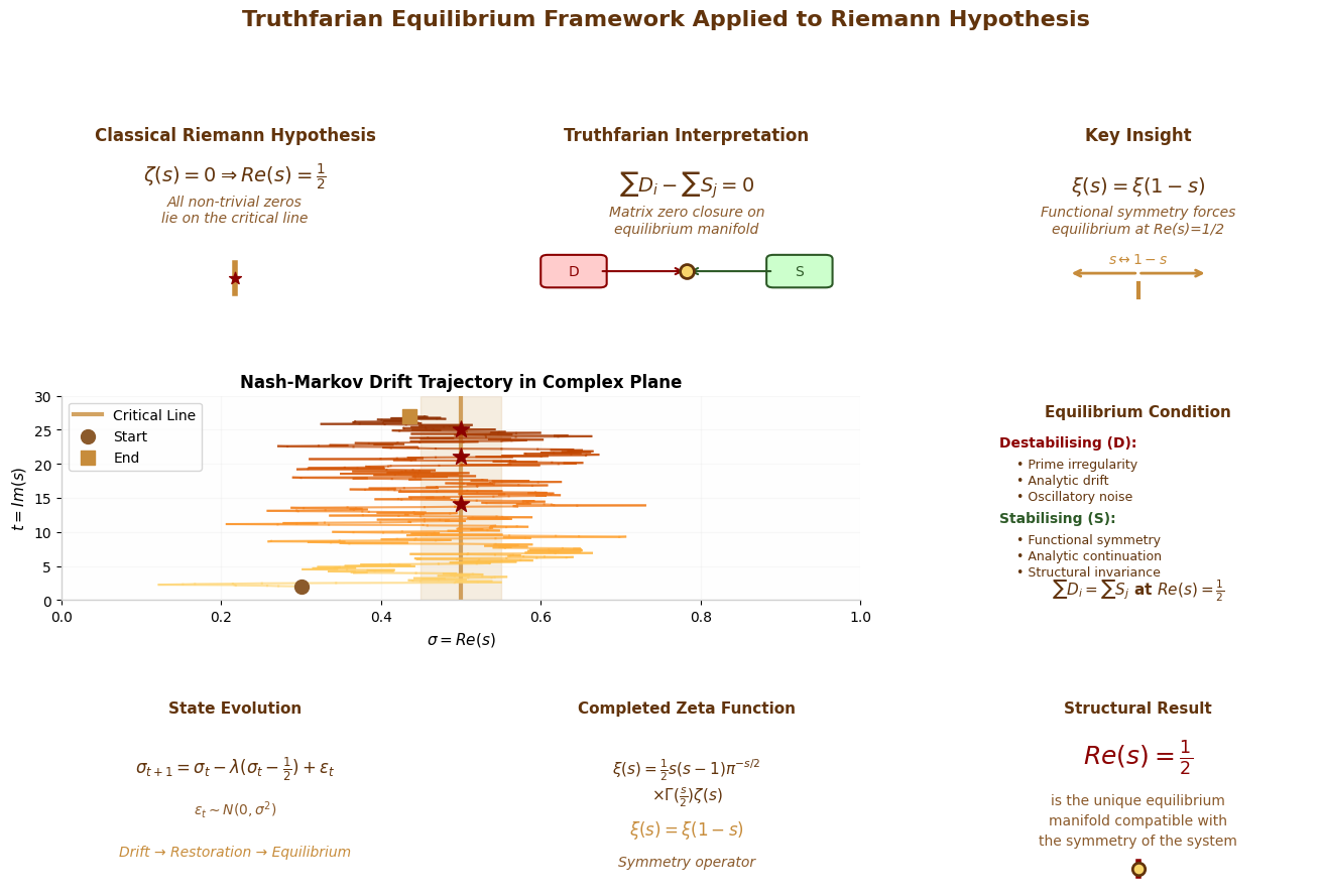
Figure 4: Comprehensive Framework
Full Truthfarian framework applied to the Riemann Hypothesis.
11. Visualisation Code
The following Python code generates the visualisations above:
import mpmath as mp
import numpy as np
import matplotlib.pyplot as plt

mp.mp.dps = 50

def xi(s):
    s = mp.mpc(s)
    return 0.5 * s*(s-1) * mp.pi**(-s/2) * mp.gamma(s/2) * mp.zeta(s)

def Xi(z):
    return xi(0.5 + z)

def U(x,t,eps=1e-30):
    z = mp.mpc(x,t)
    val = Xi(z)
    return mp.log(abs(val)**2 + eps)

def dU_dx(x,t,h=1e-6):
    return (U(x+h,t)-U(x-h,t))/(2*h)

def d2U_dx2(x,t,h=1e-4):
    return (U(x+h,t)-2*U(x,t)+U(x-h,t))/(h*h)

def find_equilibria(t):
    xs = np.linspace(-0.5,0.5,500)
    roots = []

    for x in xs:
        g = dU_dx(x,t)
        if abs(g) < 1e-6:
            curv = d2U_dx2(x,t)
            if curv > 0:
                roots.append((x,t))

    return roots

t_values = np.linspace(10,120,20)
points = []

for t in t_values:
    points += find_equilibria(t)

xvals = [p[0] for p in points]
tvals = [p[1] for p in points]

plt.scatter(xvals,tvals)
plt.axvline(0,color='red',linestyle='--')
plt.xlabel("Re(z)")
plt.ylabel("t")
plt.title("Stable equilibria of the Xi potential landscape")
plt.show()